Aleph Tutorial 4

Modulation Building Blocks

Reflecting on the first few tutorials we’ve found there’s two main elements to building a bees scene. Firstly the concept of how the scene will function, and secondly how the aleph’s various interface options are connected to those functions. While describing these functions with language is often effective, it can be difficult to turn more involved concepts (eg. Increase ENC0 to tighten normal distribution curve) into a series of connected operators to achieve that goal.

This tutorial will attempt to break down this disconnect by providing a method for visualising functional blocks, while also providing guidelines for some reusable tools. For those of you familiar with graphical programming tools (eg. MaxMSP, puredata) the drawings will probably be quite easy to understand. For those unfamiliar you should be able to grasp the drawings by keeping a few things in mind:

Signals flow from top to bottom.
INPUTs are on top, OUTPUTs are on bottom.
Anything inside a coloured box is an OPERATOR.
Values for each OP are listed to the right of the box.

Connections

For this tutorial there are no particular inputs or outputs required, as it focusses on building blocks within bees. It will be illustrative though to load aleph-waves.ldr MODULE and plug in your sound system to the audio outputs.

Low frequency oscillators

One of the most classic modulation sources is the low frequency oscillator, or LFO. It’s been used in synthesis, effects, visualisations and countless other contexts. We’ll build three LFOs with different waveshapes for a start. Each drawing below has the ‘cycle’ length set to about one second, and all are calibrated to a 0-255 output for use later in the tutorial.

The square wave LFO is the simplest of all and a good place to start. The output simply oscillates between the minimum and maximum with an even amount of time spent at each point. We can achieve this with a METRO operator acting as a clock and a TOG (or toggle) operator working as a ‘flip flop’ to alternate between zero and the value we set. To begin, create the two required operators (in yellow).

Create a METRO operator.
Create a TOG operator.

Then we need to connect the operators together. In the space between METRO and TOG you will see the words TICK and STATE which are the respective outputs and inputs of the operators. When you are connecting the operators on the OUTPUTS page you will note that this is very similar to how the routing appears on the aleph’s screen.

Connect METRO/TICK to TOG/STATE.

Now we need to set the values of the ops so they will output the range [0,255] at the rate of 1Hz, or once per second. A PERIOD of 500 will create a new tick every 500ms, or twice a second, which is perfect as our LFO has only 2 states to cycle through. Setting the TOG/MUL to 255 will force the ‘high’ state of the TOG to output 255, while the ‘low’ state will always be 0. Don’t forget to turn on the METRO with ENABLE = 1.

Set METRO/PERIOD to 500.
Set TOG/MUL to 255.
Set METRO/ENABLE to 1.

Of course we now have to send the output of our LFO somewhere in order for it to have any function, but our range of 0-255 is not very useful for most parameters in aleph-waves. We can create a simple level shifter that we will reuse throughout this tutorial. The values below will force our LFO to a 1 octave range between 130 & 260 Hz.

Create a MUL operator.
Create an ADD operator.
Connect MUL/VAL to ADD/A.
Set MUL/B to 12.
Set ADD/B to 12288.

Now we finally attach our LFO to the level shifter, and the level shifter to the frequency control of aleph-waves:

Connect TOG/VAL to MUL/A.
Connect ADD/SUM to hz0.

Next we can tackle the ramp LFO, also known as ‘sawtooth’. To do so we’ll approximate the shape by simply incrementing an ACCUM such that the value increases by a set amount until it reaches it’s maximum and wraps to zero (it’s minimum) to start counting again.

Create a METRO operator.
Create an ACCUM operator.
Connect METRO/TICK to ACCUM/INC.
Set METRO/VAL to 5.
Set METRO/PERIOD to 20.
Set ACCUM/MIN to 0.
Set ACCUM/MAX to 255.
Set ACCUM/WRAP to 1.

And then we can attach the output to our level shifter from above, and then turn on the METRO to start counting. Don’t forget to turn off the METRO from the above squarewave LFO with METRO/ENABLE = 0.

Connect ACCUM/VAL to MUL/A.
Set METRO/ENABLE to 1.

You should now be hearing the frequency ramping up over one whole octave, once per second. To explain how this works a little more, the METRO is sending a value of 5 once every 20ms, which means that it takes 1.02 seconds to count to 255. Close enough for our purposes. You can experiment with different settings for METRO/VAL and change the rate and direction at which the LFO will run. Try -5 to invert the ramp, or 1 to slow the ramp to once every ~5 seconds.

Different values for METRO/PERIOD will change the coarseness of the LFO. Lower periods will smooth out the values but also take up a lot of processing power. Depending on the context a quite steppy LFO will be fine, particularly when attaching to a DSP parameter as the ’Slew’ parameters can be used to ‘soften’ the rough edges. Try values of METRO/PERIOD = 100, and METRO/VAL = 20 to hear how steppiness is introduced at longer periods.

Now we can move onto a slightly more complex triangle waveform where the value first rises to the maximum then falls to the minimum and cycles. But first turn off the ramp LFO with METRO/ENABLE = 0.

The triangle LFO is similar to the ramp except it has to change directions when the maximum is reached. To do so we will turn ACCUM/WRAP off so that it won’t return to zero, but instead send an ‘overflow’ value out the WRAP output. We can ignore this value in our simple LFO and instead simply look at the sign (“is it positive or negative?”) to choose between -1 or +1. This value is then used to control whether the ACCUM will be counting up or down.

Create a METRO operator.
Create a MUL operator.
Create an ACCUM operator.
Connect METRO/TICK to MUL/A.
Connect MUL/VAL to ACCUM/INC.
Connect ACCUM/VAL to MUL/A (from the level shifter above).
Set METRO/VAL to 10.
Set METRO/PERIOD to 20.
Set MUL/B to 1.
Set ACCUM/MIN to 0.
Set ACCUM/MAX to 255.
Set ACCUM/WRAP to 0.

This forms the ramp creation section marked in yellow. It’s often easier to construct scenes in small blocks so you’re not bombarded with a huge number of ops to scroll through when you begin a network. Now we can create the logic section which provides the flip flop to change the direction of the LFO:

Create an IS operator.
Create a LIST2 operator.
Connect ACCUM/WRAP to IS/A.
Connect IS/GT to LIST2/INDEX.
Connect LIST2/VAL to MUL/B.
Set IS/B to 0.
Set IS/EDGE to 0.
Set LIST2/I0 to 1.
Set LIST2/I1 to -1.
Set METRO/ENABLE to 1.

This section introduces a few new operators we’ve not seen before. The IS op checks the input A against the stored B and calculates a number of comparison outputs. Here we use the GT output for ‘greater than’ functionality: when the input is above B (which is set to 0) the output is ‘1’, and when it’s below zero the output is ‘0’. This arrangement corresponds such that anytime the ACCUM hits 255 a ‘1’ will be created and anytime it hits 0 a ‘0’ will be created. We then use the simple but highly useful LIST2 object to create states for our binary input. Specifically when the ACCUM overflows 255 we want to change the direction to be negative and count down, hence LIST2/I1 = -1 and not the other way around.

Another fun trick here is that changing the LIST2/I0 and I1 values you can change the rate of the ramp on only the positive or negative side of the waveform. For I0 try values 1 to 10, and for I1 -1 to -10. If you set either value to 0, the LFO will stop at one end of the ramp and you’ll need to manually change MUL/B to a non-zero value to restart. Using this behaviour you could also create a simple envelope generator, triggered by sending a positive value to MUL/B while LIST2/I0 = 0.

Sample and Hold & Randomness

After building a few different LFO shapes we can discuss some modulation sources that operate on a ‘sampled’ basis.

In this section there won’t be specific instructions about how to create the network, but you are encouraged to build them by interpreting the drawing.

To build a random block all you’ll need is a METRO and a RANDOM operator. The RANDOM op will generate a new value between the MIN and MAX every time it receives something on the TRIG input. The METRO is set to a period of 125, or 8 times per second to provide a quickly changing value. Again the 0 to 255 limit has been used so you’ll need to attach the output to the level-shifter (MUL → ADD) from the square wave LFO section. Again make sure you’ve turned off the triangle LFO’s METRO.

The above random block functions like a sample and hold where the input is a randomly generated value. However you can use a sample and hold on other modulation sources to create a number of effects. These can be creating a deliberately ‘stepped’ output from a continuous output, or can be trigged in an ‘event oriented’ manner rather than continuously.

In the above example the METRO is again simply a clock that determines how often the input is ‘sampled’, while the GATE is being used as a simple memory cell. While GATE is usually used to control whether a signal is sent through or stopped, it can also be used in the STORE=1 mode. When you send a zero to the GATE/GATE input it will output the most recently received value to the GATED output, while a vaue of ‘1’ will open all signals through the GATE. By changing the METRO/VAL between 0 and 1, you can turn on and off the ‘sample and hold’ behaviour of GATE.

Try sending the output of the ramp or triangle LFO above into the GATE/VAL input. ENABLE the METRO and switch between METRO/VAL=0 and 1, to turn on and off the sample and hold.

Finally you will note the HISTORY operator down the bottom of the diagram. While this object has many uses it is particularly interesting to expand a sample & hold sequence. In modular synthesis this function is often known as an analog shift register. The idea is that each of the last 8 samples are simultaneously available at the output creating a bank of ‘delayed by 1’ outputs. These can be used to create ‘arabesque’ motifs or canonical sequences where multiple voices are repeated versions of previous ones.

To try out this functionality attach the GATE/GATED output to HISTORY/IN, then attach HISTORY/O0 to the level shifter from above. This will have the same effect as without HISTORY. Now we can connect O1 to another level shifter, then on to the hz1 parameter. To do so you’ll need a MUL (B=12) → ADD (B=12288) network to do the level shifting. You should then be able to hear the second oscillator following the pitch of the first. Experiment with more of these outputs to create phased pieces, and try out the AVG output for a smoothed average of the last 8 inputs.

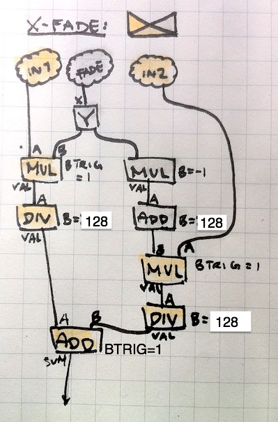
Now that we’ve seen a number of ways to create these modulation sources, here’s an interesting way to crossfade between two of them. This little block scales two inputs by an inverse amount such that when input 1 is at full level, input 2 is at zero and vice versa. It is a ‘linear’ crossfade which means that at the mid-point in the fade both inputs are scaled by half. This is also the point where our 0 to 255 range comes in handy!

Due to the nature of bees working with 16bit integers there are some ideas that need special attention. One such area is in attenuation, particularly here where we are wanting to multiply by a value between 0 and 1. Of course this is not possible! so instead we need to multiply our numbers while we do the calculation, then divide them back down. As our inputs are 0-255 (8bit) we’ll expand them by a factor of 128 which gets us very close to the highest positive integer possible, then apply the fade, and divide by 128 to return the scaling to its original level.

The crossfading mechanism itself can easily be controlled by an ENCODER (MIN=0, MAX=128, STEP=1) or another modulation source by dividing it by 2. This crossfade input from 0 to128 is sent to input 1 to multiply it by the given amount, and at the same time it is SPLIT to a MUL → ADD combination which flips the range from 128 to 0. Thus the scalers for inputs 1 and 2 operate in opposing manners.

You’ll note B_TRIG is active on the MULs that accept the crossfade control signal. This is such that even if the inputs are slowly changing sample-and-hold values they can be smoothly crossfaded between even when not changing. You may need to use B_TRIG on the final ADD if the input 2 occurs more frequently than (or independently to) input 1.

Going further

There’s already a whole lot to think about and experiment with in this tutorial but if you’re looking for more tools to experiment with the above techniques have a look at the following graphic which describes a simple probability function generator. A future tutorial will delve further into creating controlled randomness for stochastic systems, which will take this simple idea and expand it further.

And for further experiments, use the THRESH op on the output from the LFOs discussed above to split the value to 2 separate destinations based on the point in the cycle.

Next Steps

Tutorial 0: Getting Started with Bees

Tutorial 1: Making a Network

Tutorial 2: A Simple Synthesizer

Tutorial 3: Connecting a Controller

Tutorial 4: Sequencing & Modulation

Tutorial 5: Presets, Presets, Presets! →